Mastering mixed models for repeated measures and longitudinal data

The term refers to experimental designs or observational studies in which each experimental unit (or subject) is measured repeatedly over time or space. is a special case of repeated measures in which variables are measured over time (often for a comparatively long period of time) and duration itself is typically a variable of interest.

In terms of data analysis, it doesn’t really matter what type of data you have, as you can analyze both using mixed models. Remember, the key feature of both types of data is that the response variable is measured more than once on each experimental unit, and these repeated measurements are likely to be correlated.

Mixed model approaches

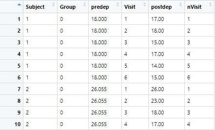
To illustrate the use of mixed model approaches for analyzing repeated measures, we’ll examine a data set from Landau and Everitt’s 2004 book, “A Handbook of Statistical Analyses using SPSS”. Here, a double-blind, placebo-controlled clinical trial was conducted to determine whether an estrogen treatment reduces post-natal depression. Sixty three subjects were randomly assigned to one of two treatment groups: placebo (27 subjects) and estrogen treatment (36 subjects). Depression scores were measured on each subject at baseline, i.e. before randomization (predep) and at six two-monthly visits after randomization (postdep at visits 1-6). However, not all the women in the trial had their depression score recorded on all scheduled visits.

In this example, the data were measured at fixed, equally spaced, time points. (Visit is time as a factor and nVisit is time as a continuous variable.) There is one between-subject factor (Group, i.e. the treatment group, either placebo or estrogen treatment), one within-subject factor (Visit or nVisit) and a covariate (predep).

Using the following plots, we can explore the data. In the first plot below, the depression scores for each subject are plotted against time, including the baseline, separately for each treatment group.

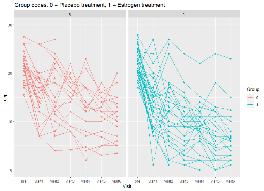
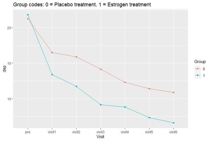
In the second plot, the mean depression score for each treatment group is plotted over time. From these plots, we can see variation among subjects within each treatment group that depression scores for subjects generally decrease with time, and on average the depression score at each visit is lower with the estrogen treatment than the placebo.

Random effects model

The simplest approach for analyzing repeated measures data is to use a random effects model with subject fitted as random. It assumes a constant correlation between all observations on the same subject. The analysis objectives can either be to measure the average treatment effect over time or to assess treatment effects at each time point and to test whether treatment interacts with time.

In this example, the treatment (Group), time (Visit), treatment by time interaction (Group:Visit) and baseline (predep) effects can all be fitted as fixed. The subject effects are fitted as random, allowing for constant correlation between depression scores taken on the same subject over time.

The code and output from fitting this model in ASReml-R 4 follows;

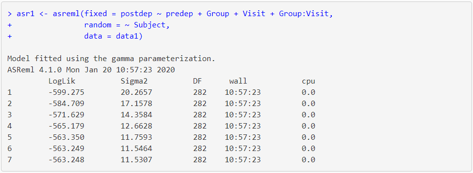
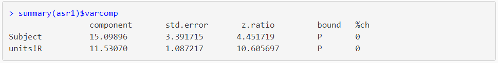
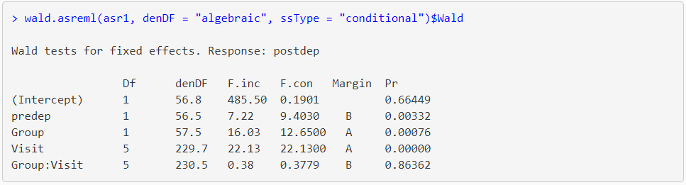
The output from summary() shows that the estimate of subject and residual variance from the model are 15.10 and 11.53, respectively, giving a total variance of 15.10 + 11.53 = 26.63. The Wald test (from the wald.asreml() table) for predep, Group and Visit are significant (probability level (Pr) ≤ 0.01). There appears to be no relationship between treatment group and time (Group:Visit) i.e. the probability level is greater than 0.05 (Pr = 0.8636).

Covariance model

In practice, often the correlation between observations on the same subject is not constant. It is common to expect that the covariances of measurements made closer together in time are more similar than those at more distant times. Mixed models can accommodate many different covariance patterns. The ideal usage is to select the pattern that best reflects the true covariance structure of the data. A typical strategy is to start with a simple pattern, such as compound symmetry or first-order autoregressive, and test if a more complex pattern leads to a significant improvement in the likelihood.

Note: using a covariance model with a simple correlation structure (i.e. uniform) will provide the same results as fitting a random effects model with random subject.

In ASReml-R 4 we use the corv() function on time (i.e. Visit) to specify uniform correlation between depression scores taken on the same subject over time.

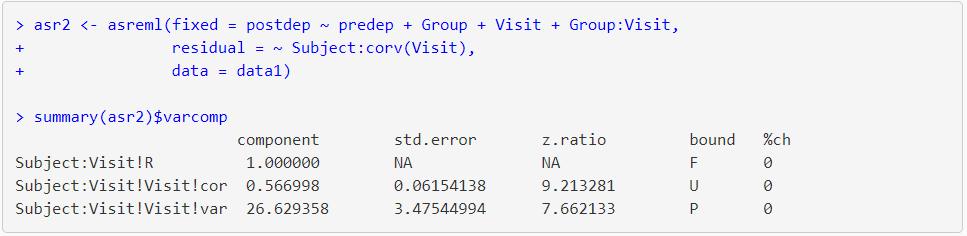
Here, the estimate of the correlation among times (Visit) is 0.57 and the estimate of the residual variance is 26.63 (identical to the total variance of the random effects model, asr1).

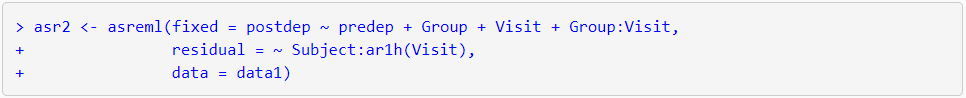
Specifying a heterogeneous first-order autoregressive covariance structure is easily done in ASReml-R 4 by changing the variance-covariance function in the residual term from corv() to ar1h().

Random coefficients model

When the relationship of a measurement with time is of interest, a random coefficients model is often appropriate. In a random coefficients model, time is considered a continuous variable, and the subject and subject by time interaction (Subject:nVisit) are fitted as random effects. This allows the slopes and intercepts to vary randomly between subjects, resulting in a separate regression line to be fitted for each subject. However, importantly, the slopes and intercepts are correlated.

The str() function of asreml() call is used for fitting a random coefficient model;

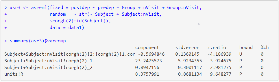
The summary table contains the variance parameter for Subject (the set of intercepts, 23.24) and Subject:nVisit (the set of slopes, 0.89), the estimate of correlation between the slopes and intercepts (-0.57) and the estimate of residual variance (8.38).

References

Brady T. West, Kathleen B. Welch and Andrzej T. Galecki (2007). Linear Mixed Models: A Practical Guide Using Statistical Software. Chapman & Hall/CRC, Taylor & Francis Group, LLC.

Brown, H. and R. Prescott (2015). Applied Mixed Models in Medicine. Third Edition. John Wiley & Sons Ltd, England.

Sabine Landau and Brian S. Everitt (2004). A Handbook of Statistical Analyses using SPSS. Chapman & Hall/CRC Press LLC.